This vignette aims at guiding the reader through the different steps of the analysis carried out in Priority effects will prevent range shifts of temperate tree species into the boreal forest.¹.

Data

Data are currently archived on Dryad at the following URL https://doi.org/10.5061/dryad.q573n5tdx and can be download using retrieveData() as follows

retrieveData()

This create a folder (by default it is input) with all datasets as .csv or .xlsx files. Once done, trees locations and regeneration files can readily be formatted with formatData(). Note that, as favuorability data are strored as .docx files,in order to use the code below it requires to convert the .docx into .csv files.

dat_abitibi <- formatData("input/abitibitrees.csv", "input/abitibiregen.csv",
  "input/abitibisubstrate.csv")
dat_lebic <- formatData("input/lebictrees.csv", "input/lebicregen.csv",
  "input/lebicsubstrate.csv",  abbr_site = "bic")
dat_sutton <- formatData("input/suttontrees.csv", "input/suttonregen.csv", "input/suttonsubstrate.csv", abbr_site = "sut")

By default all the files created will be exported as .rds file in output. Note that we stored all these data as .rda files in data (see, for instance, ?dat_abitibi).

Sites of the study

As explained in the original study, recruitment data have been measured on three different sites:

‘abi’: Abitibi
‘bic’: Le Bic
‘sut’: Sutton

The map below shows the location of those sites. For each site, extra information are available on click.

Tree species of the study

Abbreviations, names, TSN (Taxonomic Serial Number, visit the Integrated Taxonomic Information System website for more details about TSN) of the tree species considered and their respective presence in the three sites.
abbr1	abbr2	Scientific Names	TSN	abi	bic	sut
BF	ABBA	Abies balsamea	18032	TRUE	TRUE	TRUE
RM	ACRU	Acer rubrum	28728	TRUE	TRUE	FALSE
SM	ACSA	Acer saccharum	28731	TRUE	TRUE	TRUE
YB	BEAL	Betula alleghaniensis	19481	FALSE	FALSE	TRUE
WB	BEPA	Betula papyrifera	19489	TRUE	TRUE	TRUE
AB	FAGR	Fagus grandifolia	19462	FALSE	FALSE	TRUE
AS	POTR	Populus tremuloides	195773	TRUE	TRUE	TRUE

Recruitment data

A link to the dataset would be added once data are released.

Statistical models

Below are detailed the steps to reproduce our analysis.

Models

General equation

For a given species and a given year, the seeds recruitment depends on:

the fecundity of surrounding individuals of the same species;
the substrate favourability;
the neighborhood effect.

\[R_i = \text{STR}\sum_{j=1}^Sc_{i,j}f_{i,j}\sum_{k=1}^T\left(\frac{\text{DBH}_k}{30}\right)^2 \frac{1}{K}e^{-\text{DM}_{i,k}}e^{-\frac{h_i}{1-h_i}\sum_{l=1}^Ba_{i,l}}\]

Number of parameters per process

Ecological process	abbr	number of parameters
dispersion	disp	2
neighborhood effect	neigh	5
favorability	favo	1

Kernels

numb	disp	which	clip
0	–	non-significant	-
1	dc	lognormal	clip
2	d-	lognormal	no-clip
3	Dc	power-exponential	clip
4	D-	power-exponential	no-clip

Simulations

Overall strategy

For each model, we estimate the parameters through the maximization of the likelihood (actually the minimization of the likelihood log-transformed) for the corresponding data. Every model is a combination :

the site and the tree species considered;
the age of seedling taken into account (1 or 2);
whether we used a zero-inflated poisson or a regular poisson distribution;
the kernel dispersal used;
the distribution used to model seedling recruitment (zero-inflated poisson or a regular poisson).

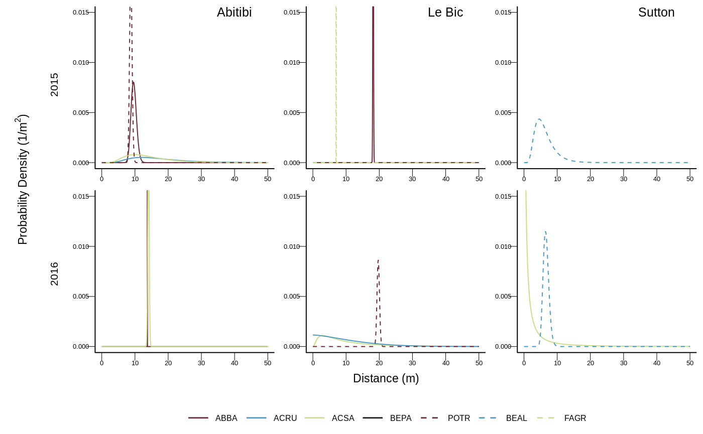
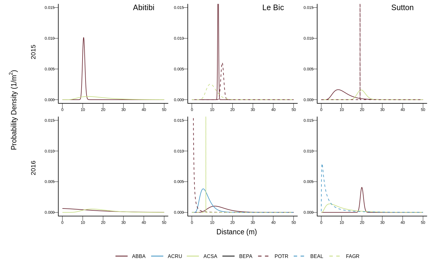
As an example, below are the 15 first models out of the 320 tested for Abies balsamea:

data(simuDesign)
# NB: each row is a model
knitr::kable(head(simuDesign, 15))

site	tree	year	age	pz	disp	favo	neigh
abi	ABBA	2015	1	TRUE	0	TRUE	TRUE
abi	ABBA	2015	1	TRUE	1	TRUE	TRUE
abi	ABBA	2015	1	TRUE	2	TRUE	TRUE
abi	ABBA	2015	1	TRUE	3	TRUE	TRUE
abi	ABBA	2015	1	TRUE	4	TRUE	TRUE
abi	ABBA	2015	1	TRUE	0	FALSE	TRUE
abi	ABBA	2015	1	TRUE	1	FALSE	TRUE
abi	ABBA	2015	1	TRUE	2	FALSE	TRUE
abi	ABBA	2015	1	TRUE	3	FALSE	TRUE
abi	ABBA	2015	1	TRUE	4	FALSE	TRUE
abi	ABBA	2015	1	TRUE	0	TRUE	FALSE
abi	ABBA	2015	1	TRUE	1	TRUE	FALSE
abi	ABBA	2015	1	TRUE	2	TRUE	FALSE
abi	ABBA	2015	1	TRUE	3	TRUE	FALSE
abi	ABBA	2015	1	TRUE	4	TRUE	FALSE

As the models we used are not linear and highly customized we optimized the likelihood with the simulated annealing algorithm implemented in GenSA².

Numerical implementation

For each row of simuDesign, columns are arguments passed to recruitmentAnalysis() in which:

parameters are computed for the simulated annealing (getParameters());
simulated annealing is performed (GenSA() from GenSA package) to minimize the likelihood (getLikelihood()).

knitr::kable(getParameters(TRUE, TRUE, TRUE, lognormal = FALSE))

	STR	Pz	scal	shap	pm	pl	pn	pd	ps	pb
start	1e+02	0.5	1.00	2	0.5	0.5	0.5	0.5	0.5	1
low	0e+00	0.0	0.02	1	0.0	0.0	0.0	0.0	0.0	0
high	1e+06	1.0	20.00	4	1.0	1.0	1.0	1.0	1.0	1000

Example

The line below (not run) allows to run for the 16^th model.

res <- launchIt(iter = 16, simu = simuDesign, mxt = 100,
  record = "output/test.txt", quiet = TRUE, path = "output/")
# value (likelihood)
res$value
# parameters value
res$par

Note that test.txt records all the values tested during the simulated algorithm and the corresponding likelihood based on which we obtain a confident interval.

getConfInt("inst/res/test.txt", simuDesign, 16, basename_out = "inst/resf_")

Figure 5

Once all models run and the best models identified, we draw figure 5 that is the dispersal kernels inferred for one year seedlings

figKernels(res_bestModels)

Similarly, we used this function to draw the same figure for 2 years seedlings (see Supplememtary Information of the paper):

figKernels(res_bestModels, age = 2)

References

Solarik et al. DOI: 2Badded↩
Y. Xiang, S. Gubian. B. Suomela, J. Hoeng (2013). Generalized Simulated Annealing for Efficient Global Optimization: the GenSA Package for R. The R Journal, Volume 5/1, June 2013. https://journal.r-project.org/archive/2013/RJ-2013-002/index.html ↩

How to reproduce the analysis

Kevin Cazelles and Kevin Solarik

2019-10-20