October 29th, 2017
R to visualize your data
Why visualize your data?
- many pieces of information at one glance
- explore your data
- make your point
Data visualization
Why use R to do it?
Workflow
## Why use R to do it?
### Workflow
Why use R to do it?
Different valuable options
Why use R to do it?
Many, many, many packages available
Why use R to do it?

Why use R to do it?
Few lines of codes
library(raster)
library(mapview)
elvBtn = getData('alt', country='BTN', path='./assets/')
mapview(elvBtn)
Why use R to do it?
Few lines of codes
Why use R to do it?
A large community
Why use R to do it?
Common plots used in meta-analyses
What do we want/need to visualize?
Effect Size (ES)
- log risk ratios,
- log odds ratios,
- …,
- non-standard ES
Studies
- by author
- by region
- by species
Effect size – Funnel plot

http://www.metafor-project.org/doku.php/plots:funnel_plot_with_trim_and_fill
Effect size – Forest plot
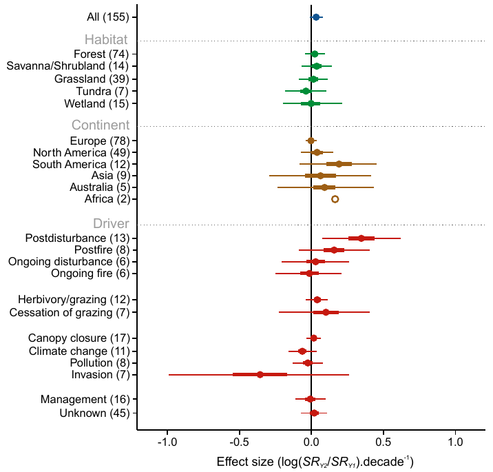
 Vellend et. al 2013
Effect size – Forest plot

http://www.metafor-project.org/doku.php/plots:forest_plot_with_subgroups
Effect size – Radial plot

Effect size – L’Abbé plot

Effect size – relevant categories
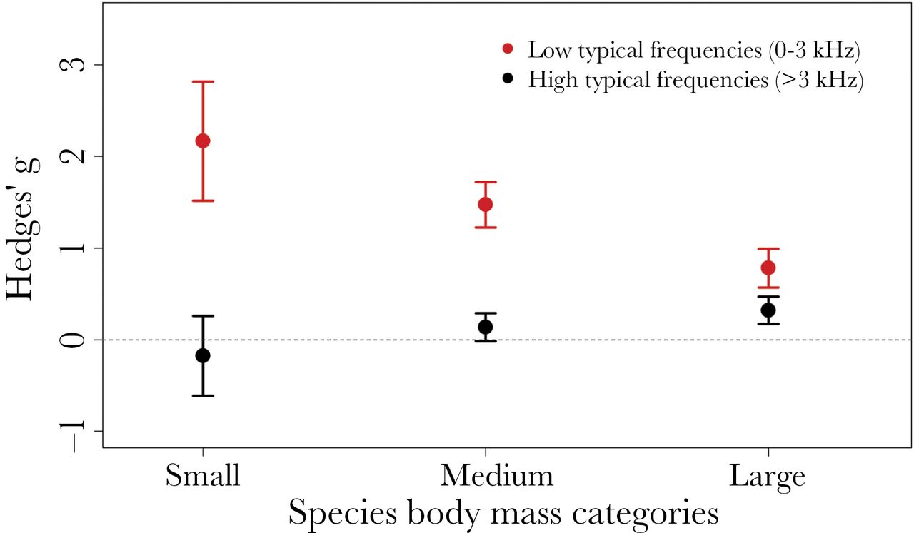
Roca et al. 2016
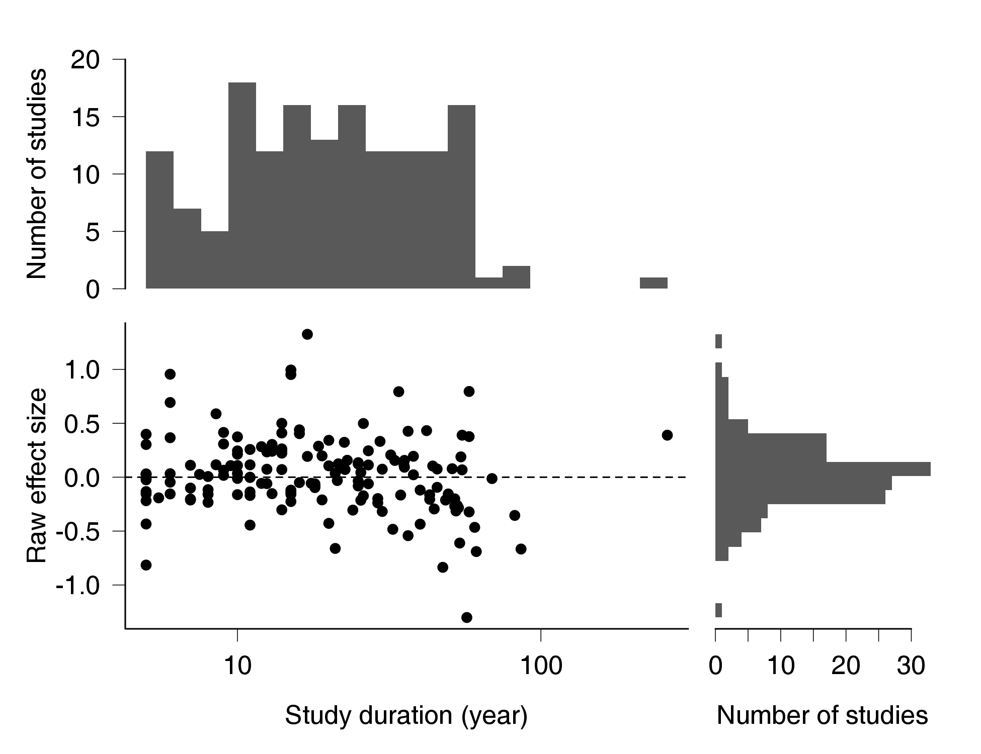
Number of Study & effect size
Vellend et al. 2013
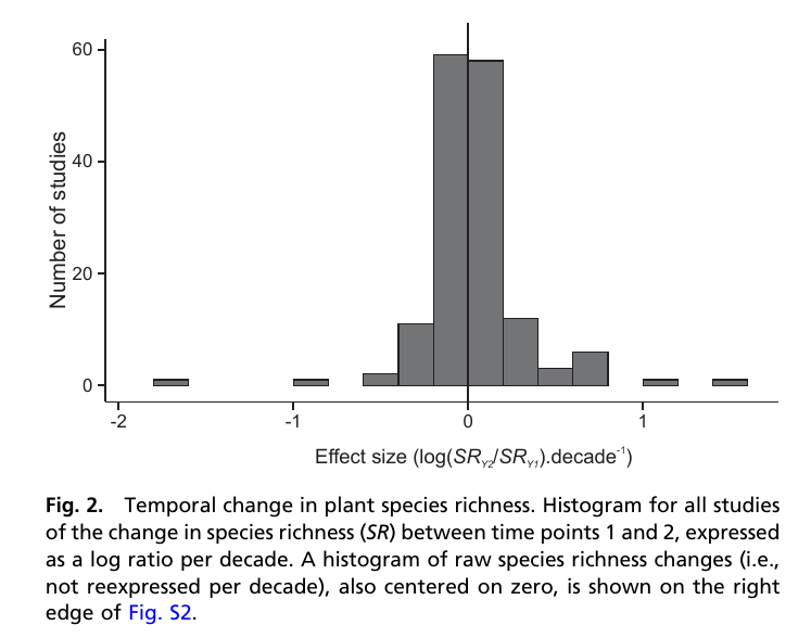
Number of Study & geography
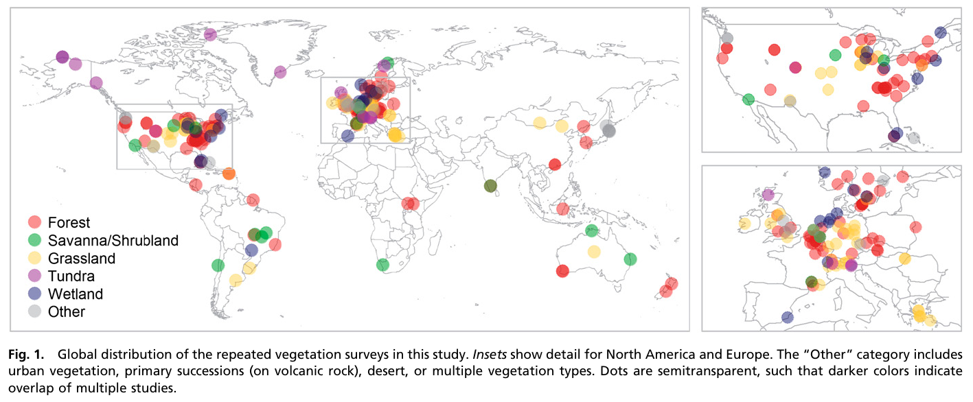
Vellend et al. 2013
Common plots used in meta-analyses with R
R packages for meta-analyses
install.packages("ctv"); ctv::install.views("MetaAnalysis")
Meta vs Metafor – briefly

Meta vs Metafor – briefly
Meta vs Metafor – support
Guido Schwarzer author of
metaSchwarzer, Guido, James R. Carpenter, and Gerta Rücker. Meta-Analysis with R.
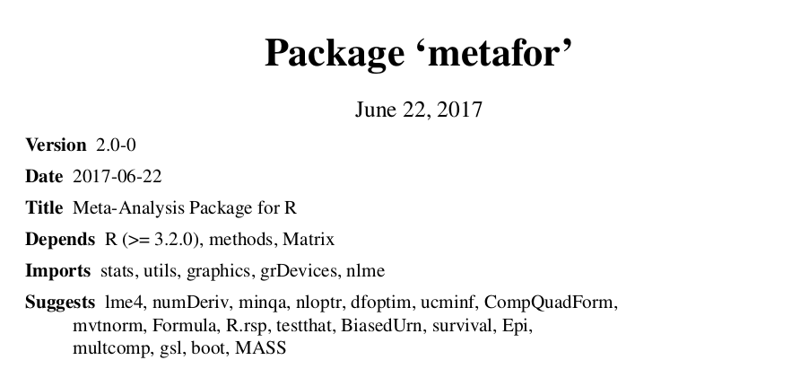
Wolfgang Viechtbauer author
metafor
Meta – workflow
metabin()
Arguments:

 event.e: Number of events in experimental group.
     n.e: Number of observations in experimental group.
 event.c: Number of events in control group.
     n.c: Number of observations in control group.
Meta – workflow
metabin()metagen()
Arguments:

      TE: Estimate of treatment effect.
    seTE: Standard error of treatment estimate.
Meta – workflow
meta:
- `metabin()` / `metagen()`
- `funnel`, `forest`, ...
install.packages('meta')
library(meta)
data(Olkin95)
# ?Olkin95
meta1 <- metabin(event.e, n.e, event.c, n.c,
                  data=Olkin95, subset=c(41,47,51,59),
                  sm="RR", method="I",
                  studlab=paste(author, year))

forest(meta1)
Meta – workflow
| author | year | event.e | n.e | event.c | n.c |
|---|---|---|---|---|---|
| Fletcher | 1959 | 1 | 12 | 4 | 11 |
| Dewar | 1963 | 4 | 21 | 7 | 21 |
| Lippschutz | 1965 | 6 | 43 | 7 | 41 |
| European 1 | 1969 | 20 | 83 | 15 | 84 |
| European 2 | 1971 | 69 | 373 | 94 | 357 |
| Heikinheimo | 1971 | 22 | 219 | 17 | 207 |
Meta – workflow

Metafor – workflow
Metafor – workflow
Calculate effect size:
escalc()Perform analysis:
rma()Plots:
funnel(),forest(),labbe(), …
Metafor – example
install.packages('metafor')
library('metafor')
Metafor – example
r<-c(0.5,0.6,0.4,0.2,0.7,0.45)
n<-c(40,90,25,400,60,50)
studynames<-c(1,2,3,4,5,6)
b<-data.frame(r,n,studynames)
eszcor <- escalc(measure="ZCOR", ri=r, ni=n, data=b)
FEmodel<-rma(yi=yi, vi=vi, data=eszcor, method="FE")
#forest plot fixed-effect model: pooled effect size,
forest(FEmodel)
Metafor – example
r<-c(0.5,0.6,0.4,0.2,0.7,0.45)
n<-c(40,90,25,400,60,50)
studynames<-c(1,2,3,4,5,6)
b<-data.frame(r,n,studynames)
Metafor – example
knitr::kable(head(b))
| r | n | studynames |
|---|---|---|
| 0.50 | 40 | 1 |
| 0.60 | 90 | 2 |
| 0.40 | 25 | 3 |
| 0.20 | 400 | 4 |
| 0.70 | 60 | 5 |
| 0.45 | 50 | 6 |
Metafor – example
eszcor <- escalc(measure="ZCOR", ri=r, ni=n, data=b)
class(eszcor)
R>> [1] "escalc" "data.frame"
Metafor – example
FEmodel<-rma(yi=yi, vi=vi, data=eszcor, method="FE")
class(FEmodel)
R>> [1] "rma.uni" "rma"
Metafor – example
forest(FEmodel)

Metafor – example
forest(FEmodel,transf=transf.ztor)

Metafor – example
funnel(FEmodel, yaxis="vinv", main="Inverse Sampling Variance")

Pros and Cons
Pros
- do everything for you
- good-looking plots with few lines of code
Cons
- standard ES
- not fully customizable
- not for ecologists?
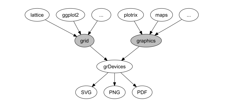
Custom your plot
graphics or grid?
Few tips
par()plot(),barplot(),funnel()
npt <- 15
vecX <- 1:npt
vecY <- runif(length(vecX))
plot(vecX, vecY)

plot(vecX, vecY, xlim=c(0,15)+.5)

plot(vecX, vecY, xlim=c(0,15)+.5, pch=19)

plot(vecX, vecY, xlim=c(0,15)+.5, pch=19, col="#0f7aa2")

plot(vecX, vecY, xlim=c(0,15)+.5, pch='S', col="#0f7aa2")

plot(vecX, vecY, xlim=c(0,15)+.5, type='h', col="#0f7aa2")

plot(vecX, vecY, xlim=c(0,15)+.5, type='h', col="#0f7aa2", lwd=12)

par(lend=2); plot(vecX, vecY, xlim=c(0,15)+.5, type='h', col="#0f7aa2", lwd=12)

par(las=1)
plot(vecX, vecY, xlim=c(0,15)+.5, pch=19, col="#0f7aa2")

par(las=1)
plot(vecX, vecY, xlim=c(0,15)+.5, pch=19, col="#0f7aa2")
abline(v=c(0.5,15.5), lty=2)

par(las=1, xaxs='i')
plot(vecX, vecY, xlim=c(0,15)+.5, pch=19, col="#0f7aa2")
abline(v=c(0.5,15.5), lty=2)

vCol <- rep(1, npt)
vCol[c(2,5,8,9)] <- 2
vSize <- 1+2*runif(npt)
par(las=1, xaxs='i')
plot(vecX, vecY, xlim=c(0,15)+.5, pch=19, col=c("#0f7aa2", '#a70d72')[vCol])

par(las=1, xaxs='i')
plot(vecX, vecY, xlim=c(0,15)+.5, pch=19, col=c("#0f7aa2", '#a70d72')[vCol], cex=vSize)

par(las=1, xaxs='i')
plot(vecX, vecY, xlim=c(0,15)+.5, pch=19, col=c("#0f7aa2", '#a70d72')[vCol], cex=vSize)
abline(lm(vecY~vecX), col=2)

par(las=1, xaxs='i', mfrow=c(2,2))
for (i in 1:4){
  plot(vecX, vecY, xlim=c(0,15)+.5, pch=19, col=c("#0f7aa2", '#a70d72')[vCol], cex=vSize)
  mtext(3, at=2, text=LETTERS[i], line=.5, cex=1.2)
}

par(las=1, xaxs='i', mfrow=c(2,2), mar=c(2,2,2,1), oma=c(3,3,0,0), mgp=c(1,0.8,0))
##--
for (i in 1:4){
  plot(vecX, vecY, xlim=c(0,15)+.5, pch=19, col=c("#0f7aa2", '#a70d72')[vCol],
    cex=vSize, ann=FALSE)
  mtext(3, at=1, text=LETTERS[i], line=.5, cex=1.2)
}
##--
mtext(1, text='Time', outer=T, line=1, cex=1.4)
par(las=0)
mtext(2, text='Variable', outer=T, line=1, cex=1.4)

layout(matrix(c(2,1,0,3), 2), widths=c(1,.5), heights=c(.5,1))
layout.show(3)

layout(matrix(c(1,2,0,3), 2), widths=c(1,.5), heights=c(.6,1))
par(mar=c(2, 4, 2, 1), las=1)
for (i in 1:3){
  plot(vecX, vecY, xlim=c(0,15)+.5, pch=19, col=c("#0f7aa2", '#a70d72')[vCol],
    cex=vSize, ann=FALSE)
  mtext(3, at=1, text=LETTERS[i], line=.5, cex=1.2)
}

Example funnel plot
funnel(FEmodel, yaxis="vinv", main="Inverse Sampling Variance")

Example funnel plot
par(las=1, mar=c(5,6,4,1), mgp=c(4,1,0))
funnel(FEmodel, yaxis="vinv", main="Inverse Sampling Variance", col="#0f7aa2",
back='white')
legend('topright', legend='mypoints', pch=19, col="#0f7aa2", bty='n')
Example funnel plot

Questions?
Let’s practice
Reproduce figures from….
1- Roca et al. 2016
2- Vellend et al. 2013
Data available on line as well Dataset S1
Roca et al. 2016
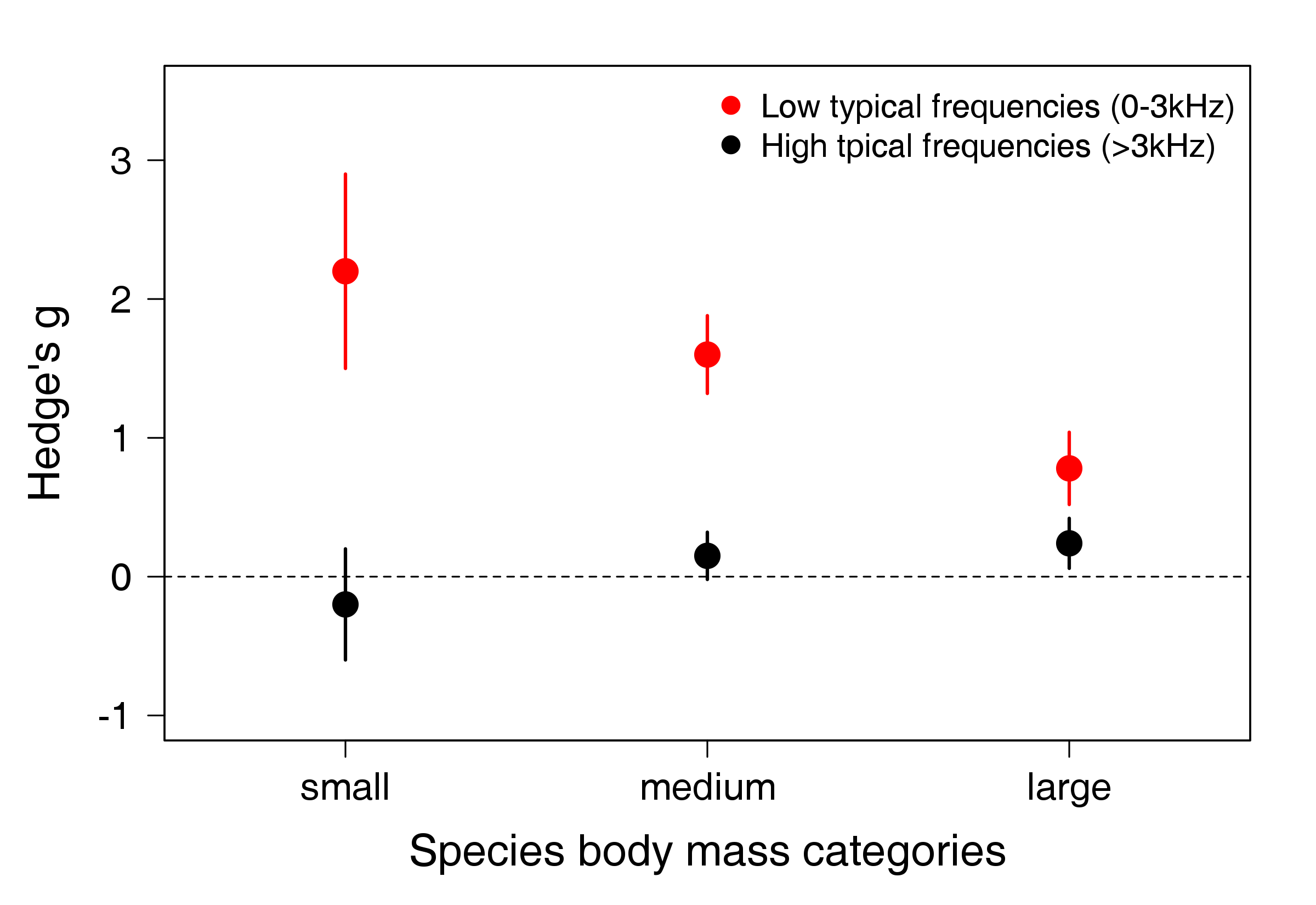
Figure 1 from Roca et al. 2016
Vellend et al. 2013
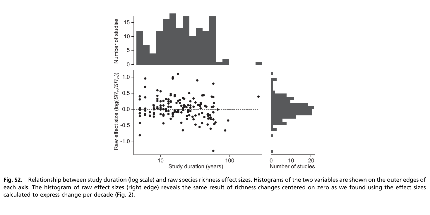
Figure S2 Vellend et al. 2013
Roca et al. 2016 – Solution
Find the R script I created to reproduce this figure here
Amanda Young kindly sent me her version using ggplot2
Roca et al. 2016 – Solution
Roca et al. 2016
 KevCaz
Roca et al. 2016 – Solution
Roca et al. 2016
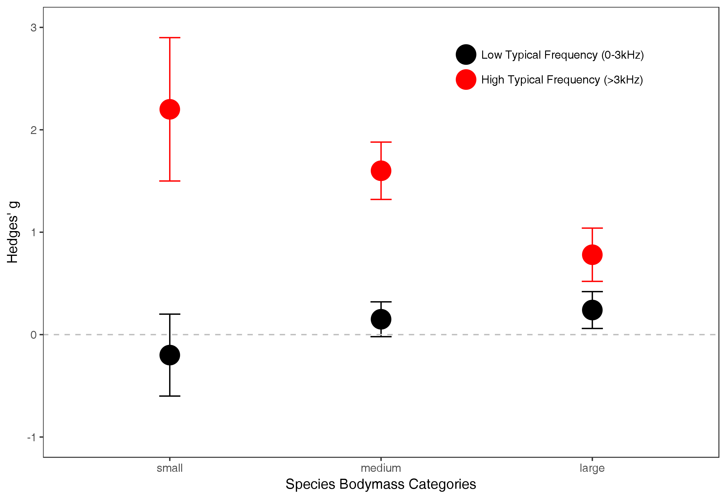 Amanda Young
Figure S2 Vellend et al. 2013 – Solution
Find the R script I created to reproduce this figure here
Figure S2 Vellend et al. 2013 – Solution
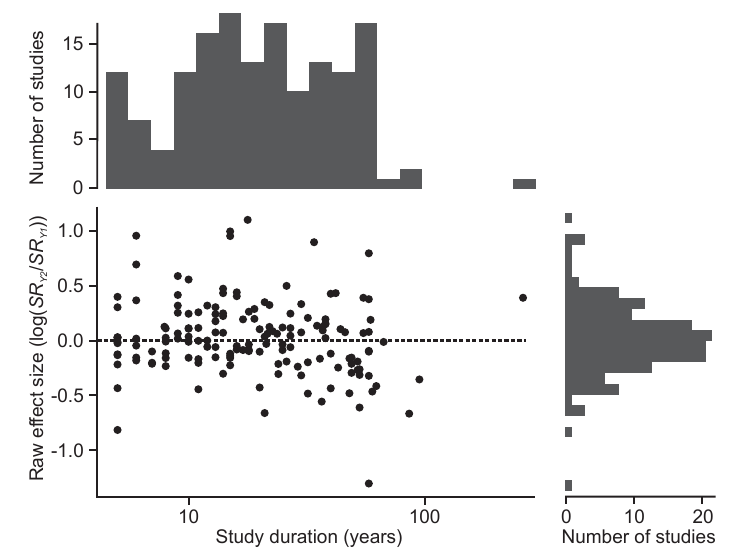 Vellend et al. 2013
 KevCaz
Extra
Network of co-authors
To create the network that follows:
1- data available on Github;
2- R script available on Github.
Resources
Useful links
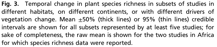
2 books:
Chen, Ding-Geng, and Karl E. Peace. Applied Meta-Analysis with R. Chapman & Hall/CRC Biostatistics Series. Boca Raton: CRC Press/Taylor & Francis Group, 2013. + companion website
Schwarzer, Guido, James R. Carpenter, and Gerta Rücker. Meta-Analysis with R. Use R! Cham: Springer International Publishing, 2015. https://doi.org/10.1007/978-3-319-21416-0.